Build efficient optimal control software, with minimal effort.
CasADi is an open-source tool for nonlinear optimization and algorithmic differentiation.
It facilitates rapid — yet efficient — implementation of different methods for numerical optimal control, both in an offline context and for nonlinear model predictive control (NMPC).
Algorithmic Differentiation (AD)
These expression graphs, encapsulated in Function objects, can be evaluated in a virtual machine or be exported to stand-alone C code.

import casadi.*


% Create scalar/matrix symbols
x = MX.sym('x',5);

% Compose into expressions
y = norm(x,2);

% Sensitivity of expression -> new expression
grad_y = gradient(y,x)

% Create a Function to evaluate expression
f = Function('f',{x},{grad_y});

% Evaluate numerically
grad_y_num = f([1;2;3;4;5])
from casadi import *
# Create scalar/matrix symbols
x = MX.sym('x',5)
# Compose into expressions
y = norm_2(x)
# Sensitivity of expression -> new expression
grad_y = gradient(y,x);
# Create a Function to evaluate expression
f = Function('f',[x],[grad_y])
# Evaluate numerically
grad_y_num = f([1,2,3,4,5]);#include <casadi/casadi.hpp>
using namespace casadi;
// Create scalar/matrix symbols
MX x = MX::sym("x",5,1);
// Compose into expressions
MX y = norm_2(x);
// Sensitivity of expression -> new expression
MX grad_y = gradient(y,x);
// Create a Function to evaluate expression
Function f = Function("f",{x},{grad_y});
// Evaluate numerically
std::vector<DM> grad_y_num = f(DM({1,2,3,4,5}));Dynamic systems
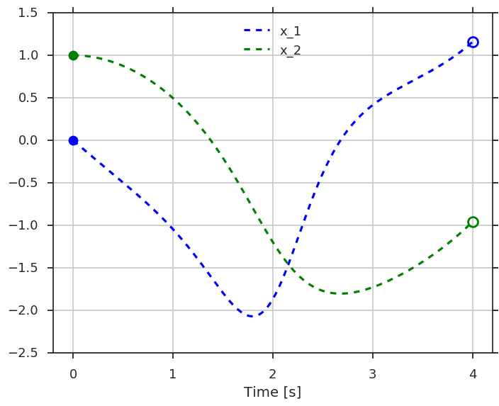
$$ \begin{align} \left\{ \begin{array}{ccll} \dot{x}_1 &=& (1-x_2^2) \, x_1 - x_2, \quad &x_1(0)=0 \\ \dot{x}_2 &=& x_1, \quad &x_2(0)=1 \end{array} \right. \end{align} $$
import casadi.*


x = MX.sym('x',2); % Two states

% Expression for ODE right-hand side
z = 1-x(2)^2;
rhs = [z*x(1)-x(2);x(1)];

ode = struct;    % ODE declaration
ode.x   = x;     % states
ode.ode = rhs;   % right-hand side

% Construct a Function that integrates over 4s
F = integrator('F','cvodes',ode,0,4);

% Start from x=[0;1]
res = F('x0',[0;1]);

disp(res.xf)

% Sensitivity wrt initial state
res = F('x0',x);
S = Function('S',{x},{jacobian(res.xf,x)});

disp(S([0;1]))
x = MX.sym('x',2); # Two states
# Expression for ODE right-hand side
z = 1-x[1]**2
rhs = vertcat(z*x[0]-x[1],x[0])
ode = {} # ODE declaration
ode['x'] = x # states
ode['ode'] = rhs # right-hand side
# Construct a Function that integrates over 4s
F = integrator('F','cvodes',ode,0,4)
# Start from x=[0;1]
res = F(x0=[0,1])
print(res["xf"])
# Sensitivity wrt initial state
res = F(x0=x)
S = Function('S',[x],[jacobian(res["xf"],x)])
print(S([0,1]))#include <casadi/casadi.hpp>
using namespace casadi;
MX x = MX::sym("x",2); // Two states
// Expression for ODE right-hand side
MX z = 1-pow(x(1),2);
MX rhs = vertcat(z*x(0)-x(1),x(0));
MXDict ode; // ODE declaration
ode["x"] = x; // states
ode["ode"] = rhs; // right-hand side
// Construct a Function that integrates over 4s
Function F = integrator("F","cvodes",ode,0,4);
// Start from x=[0;1]
DMDict res = F(DMDict{{"x0",std::vector<double>{0,1}}});
std::cout << res["xf"] << std::endl;
// Sensitivity wrt initial state
MXDict ress = F(MXDict{{"x0",x}});
Function S("S",{x},{jacobian(ress["xf"],x)});
std::cout << S(DM(std::vector<double>{0,1}));Initial value problems in ordinary or differential-algebraic equations (ODE/DAE) can be calculated using explicit or implicit Runge-Kutta methods or interfaces to IDAS/CVODES from the SUNDIALS suite. Derivatives are calculated using sensitivity equations, up to arbitrary order.
Problem class:
$$ \begin{aligned} \dot{x} &= f_{\text{ode}}(t,x,z,p), \qquad x(0) = x_0 \\ 0 &= f_{\text{alg}}(t,x,z,p) \end{aligned} $$
Nonlinear and quadratic programming
Nonlinear programs (NLPs), possibly with integer variables (MINLP), can be solved using block structure or general sparsity exploiting sequential quadratic programming (SQP) or interfaces to IPOPT/BONMIN, BlockSQP, WORHP, KNITRO, SNOPT, SLEQP, and Alpaqa. Solution sensitivities, up to arbitrary order, can be calculated analytically. Quadratic programs (QPs), possibly with integer variables (MIQP), can be solved using a primal-dual active-set method [3] or interfaces to CPLEX, GUROBI, HPIPM, OOQP, qpOASES or HiGHS.
Problem class: $$ \begin{array}{cc} \begin{array}{c} \text{minimize:} \\ x \end{array} & f(x,p) \\ \begin{array}{c} \text{subject to:} \end{array} & \begin{array}{rcl} x_{\textrm{lb}} \le & x & \le x_{\textrm{ub}} \\ g_{\textrm{lb}} \le &g(x,p)& \le g_{\textrm{ub}} \end{array} \end{array} $$
$$ \begin{equation} \begin{array}{cl} \underset{\begin{array}{c}x, y, z\end{array}}{\text{minimize}} \quad & x^2 + 100 \, z^2 \\ \text{subject to} \quad & z+(1-x)^2 - y = 0 \end{array} \end{equation} $$
import casadi.*


% Symbols/expressions
x = MX.sym('x');
y = MX.sym('y');
z = MX.sym('z');
f = x^2+100*z^2;
g = z+(1-x)^2-y;

nlp = struct;            % NLP declaration
nlp.x = [x;y;z];         % decision vars
nlp.f = f;               % objective
nlp.g = g;               % constraints

% Create solver instance
F = nlpsol('F','ipopt',nlp);

% Solve the problem using a guess
F('x0',[2.5 3.0 0.75],'ubg',0,'lbg',0)
from casadi import *
# Symbols/expressions
x = MX.sym('x')
y = MX.sym('y')
z = MX.sym('z')
f = x**2+100*z**2
g = z+(1-x)**2-y
nlp = {} # NLP declaration
nlp['x']= vertcat(x,y,z) # decision vars
nlp['f'] = f # objective
nlp['g'] = g # constraints
# Create solver instance
F = nlpsol('F','ipopt',nlp);
# Solve the problem using a guess
F(x0=[2.5,3.0,0.75],ubg=0,lbg=0)#include <casadi/casadi.hpp>
using namespace casadi;
// Symbols/expressions
MX x = MX::sym("x");
MX y = MX::sym("y");
MX z = MX::sym("z");
MX f = pow(x,2)+100*pow(z,2);
MX g = z+pow(1-x,2)-y;
MXDict nlp; // NLP declaration
nlp["x"]= vertcat(x,y,z); // decision vars
nlp["f"] = f; // objective
nlp["g"] = g; // constraints
// Create solver instance
Function F = nlpsol("F","ipopt",nlp);
// Solve the problem using a guess
F(DMDict{{"x0",DM({2.5,3.0,0.75})},{"ubg",0},{"lbg",0}});Composition of the above
import casadi.*


x = MX.sym('x',2); % Two states
p = MX.sym('p');   % Free parameter

% Expression for ODE right-hand side
z = 1-x(2)^2;
rhs = [z*x(1)-x(2)+2*tanh(p);x(1)];

% ODE declaration with free parameter
ode = struct('x',x,'p',p,'ode',rhs);

% Construct a Function that integrates over 1s
F = integrator('F','cvodes',ode,0,1);

% Control vector
u = MX.sym('u',5,1);

x = [0;1]; % Initial state
for k=1:5
  % Integrate 1s forward in time:
  % call integrator symbolically
  res = F('x0',x,'p',u(k));
  x = res.xf;
end

% NLP declaration
nlp = struct('x',u,'f',dot(u,u),'g',x);

% Solve using IPOPT
solver = nlpsol('solver','ipopt',nlp);
res = solver('x0',0.2,'lbg',0,'ubg',0);

plot(full(res.x))
from casadi import *
from matplotlib.pyplot import plot, show
x = MX.sym('x',2) # Two states
p = MX.sym('p') # Free parameter
# Expression for ODE right-hand side
z = 1-x[1]**2;
rhs = vertcat(z*x[0]-x[1]+2*tanh(p),x[0])
# ODE declaration with free parameter
ode = {'x':x,'p':p,'ode':rhs}
# Construct a Function that integrates over 1s
F = integrator('F','cvodes',ode,0,1)
# Control vector
u = MX.sym('u',4,1)
x = [0,1] # Initial state
for k in range(4):
# Integrate 1s forward in time:
# call integrator symbolically
res = F(x0=x,p=u[k])
x = res['xf']
# NLP declaration
nlp = {'x':u,'f':dot(u,u),'g':x}
# Solve using IPOPT
solver = nlpsol('solver','ipopt',nlp)
res = solver(x0=0.2,lbg=0,ubg=0)
plot(res['x'])
show()#include <casadi/casadi.hpp>
using namespace casadi;
MX x = MX::sym("x",2); // Two states
MX p = MX::sym("p"); // Free parameter
// Expression for ODE right-hand side
MX z = 1-pow(x(1),2);
MX rhs = vertcat(z*x(0)-x(1)+2*tanh(p),x(0));
// ODE declaration with free parameter
MXDict ode = {{"x",x},{"p",p},{"ode",rhs}};
// Construct a Function that integrates over 1s
Function F = integrator("F","cvodes",ode,0,1);
// Control vector
MX u = MX::sym("u",4,1);
x = DM(std::vector<double>{0,1}); // Initial state
for (int k=0;k<4;++k) {
// Integrate 1s forward in time:
// call integrator symbolically
MXDict res = F({{"x0",x},{"p",u(k)}});
x = res["xf"];
}
// NLP declaration
MXDict nlp = {{"x",u},{"f",dot(u,u)},{"g",x}};
// Solve using IPOPT
Function solver = nlpsol("solver","ipopt",nlp);
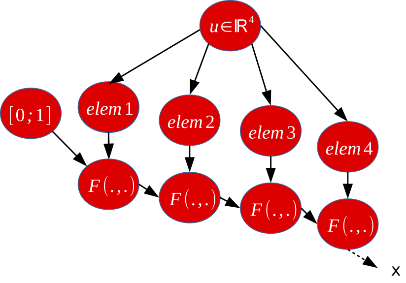
DMDict res = solver(DMDict{{"x0",0.2},{"lbg",0},{"ubg",0}});CasADi offers a rich set of differentiable operations for its matrix-valued expression graphs, including common matrix-valued operations, serial or parallel function calls, implicit functions, integrators, spline-based lookup tables, and external codes.
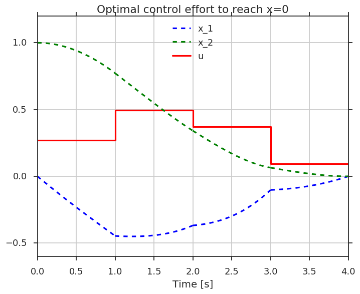
These building blocks allow the user to code a wide variety of optimal control problem (OCP) formulations.
For example, a single shooting code can be created by embedding a call to an integrator in an NLP declaration.
Applications
CasADi saves time prototyping formulations, solving complex engineering problems, and building professional optimization tools.
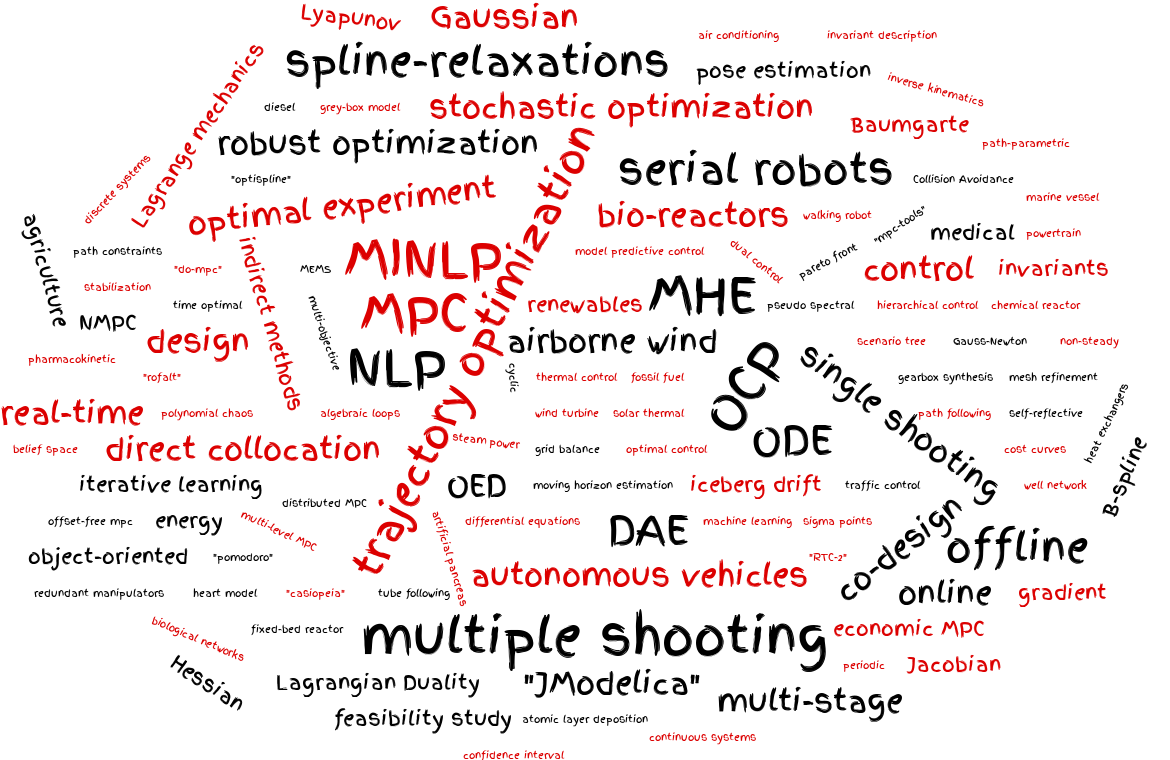
The landscape of its academic and industrial applications is diverse:
- trajectory optimization
- optimal control
- OCP
- moving horizon estimation
- MHE
- model predictive control
- MPC
- NLP
- MINLP
- ODE
- differential equations
- algebraic loops
- DAE
- optimal experiment
- OED
- pseudo spectral
- direct collocation
- single shooting
- multiple shooting
- indirect methods
- machine learning
- distributed MPC
- multi-objective
- pareto front
- robust optimization
- scenario tree
- hierarchical control
- sigma points
- design
- control
- co-design
- stochastic optimization
- multi-level MPC
- time optimal
- path following
- iterative learning
- Gauss-Newton
- energy
- medical
- stabilization
- cost curves
- grey-box model
- Collision Avoidance
- Lagrangian Duality
- economic MPC
- NMPC
- self-reflective
- real-time
- offline
- online
- Lagrange mechanics
- object-oriented
- multi-stage
- path constraints
- non-steady
- periodic
- cyclic
- feasibility study
- offset-free mpc
- Gaussian
- belief space
- continuous systems
- discrete systems
- redundant manipulators
- inverse kinematics
- Jacobian
- Hessian
- gradient
- Lyapunov
Examples of software with a CasADi backend: JModelica.org, omg-tools, MPC-tools, RTC-tools, openocl.org, rockit, yop, do-mpc, hilo-mpc, MATMPC, Optimization Engine, acados, nosnoc, OpTaS, csnlp, nmpyc, OpenAP Trajectory Optimizer, Alpaqa, SIPPY, Monomers to Polymers (m2p), MPOPT, AeroSandbox, Pymoca, L4CasADi (PyTorch coupling), Adam (Rigid-body dynamics), urdf2casadi, mopeds.
Ready to try?
Jump right in by getting CasADi and exploring the example pack, joining a workshop or online course, or watching a small tutorial.
Keep informed
Subscribe to our newsletter or follow us on the social media links below.