Sensitivities of parametric NLP
Estimated reading time: 3 minutesIn this post, we explore the parametric sensitivities of a nonlinear program (NLP). While we use ‘Opti stack’ syntax for modeling, differentiability of NLP solvers works all the same without Opti.
Parametric nonlinear programming
Let’s start by defining an NLP that depends on a parameter $p \in \mathbb{R}$ that should not be optimized for: $$ \begin{align} \displaystyle \underset{x,y} {\text{minimize}}\quad &\displaystyle (1-x)^2+0.2(y-x^2)^2 \newline \text{subject to} \, \quad & \frac{p^2}{4} \leq (x+0.5)^2+y^2 \leq p^2 \newline & x\geq 0 \end{align} $$
For each choice of $p$, we have a different optimization problem, with a corresponding solution pair $(x^\star(p),y^\star(p))$.
The figure below visualizes this problem and its solution pair for three different values of $p$:
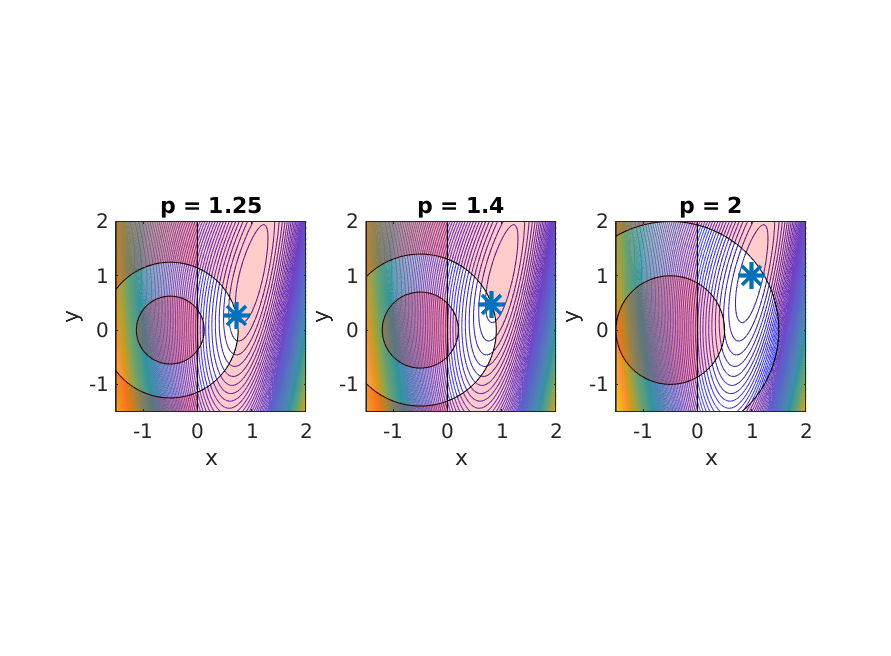
Parametric NLP visualized for different p
We’d like to investigate how the NLP solution varies with $p$. To simplify visualization, let’s consider a projection of the solution pair to a scalar:
$$ z: (x,y) \mapsto y-x $$
Instead of working with the $x^\star$ notation, let’s define the parametric solution function $M(p): \mathbb{R} \mapsto \mathbb{R}^2$: $$ M(p):= \begin{align} \displaystyle \underset{x,y} {\text{argmin}}\quad &\displaystyle (1-x)^2+0.2(y-x^2)^2 \newline \text{subject to} \, \quad & \frac{p^2}{4} \leq (x+0.5)^2+y^2 \leq p^2 \newline & x\geq 0 \end{align} $$
For a range of different $p$ values, we consider $z(M(p))$:
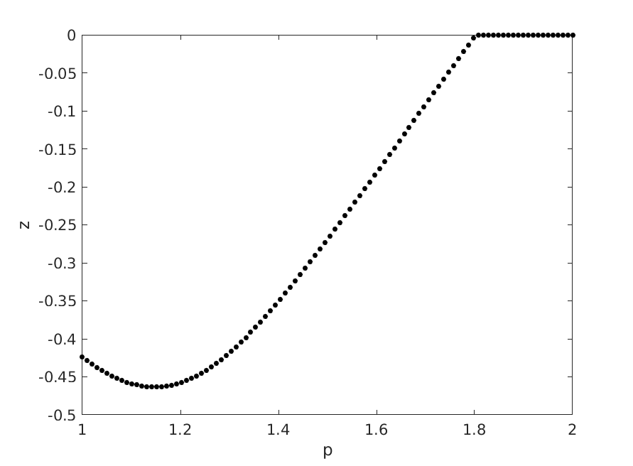
Parametric solution curve for sampled in p
Notice how the slope of the curve makes a jump. This happens when the set of active constraints changes.
The goal of the remainder is to obtain Taylor approximations of this curve, without resorting to sampling and finite differences.
Parametric solution as CasADi Function
We use Opti to model the problem:
opti = Opti();

x = opti.variable();
y = opti.variable();

xy = [x;y];
p = opti.parameter();

opti.minimize((1-x)^2 + 0.2*(y-x^2)^2);
opti.subject_to(x>=0);
opti.subject_to((p/2)^2 <= (x+0.5)^2+y^2 <= p^2);
We use to_function to represent the parametric solution function $M$ as a regular CasADi Function.
This Function has an Ipopt solver embedded.
opts = struct;
opts.ipopt.print_level = 0;
opts.print_time = false;
opti.solver('ipopt',opts);

M = opti.to_function('M',{p},{xy});
With M in place, we can easily recreate the figure above by solving 100 Ipopt problems:
z = @(xy) xy(2,:)-xy(1,:);

pvec = linspace(1,2,100);
S = full(M(pvec));

plot(pvec,z(S));
Parametric sensitivities
Ipopt is a very robust nonlinear optimizer: it finds solutions from bad initial guesses. SQPMethod+QRQP is more fragile, but delivers more accuracy in dual variables when it converges. We make a combination of the two to obtain accurate sensitivity information.
Let’s create a CasADi Function Z that computes the projected solution given p and an initial guess for decision variables.
opts = struct;
opts.qpsol = 'qrqp';
opti.solver('sqpmethod',opts);

Z = opti.to_function('Z',{p,xy},{z(xy)});
Calling that Function Z symbolically allows us to perform algorithmic differentiation on the resultant expression:
zp = Z(p,xy);
j = jacobian(zp,p);
h = hessian(zp,p);

Z_taylor = Function('Z_taylor',{p,xy},{zp,j,h});
Evaluate Z_taylor numerically to be able to plot some nice second-order approximations onto the previous plot:
for p0 =  [1.25,1.4,2]
    [F,J,H] = Z_taylor(p0,M(p0));
    plot(p_lin,full(F),'x');
    plot(t,full(F+J*(t-p0)+1/2*H*(t-p0).^2));
end
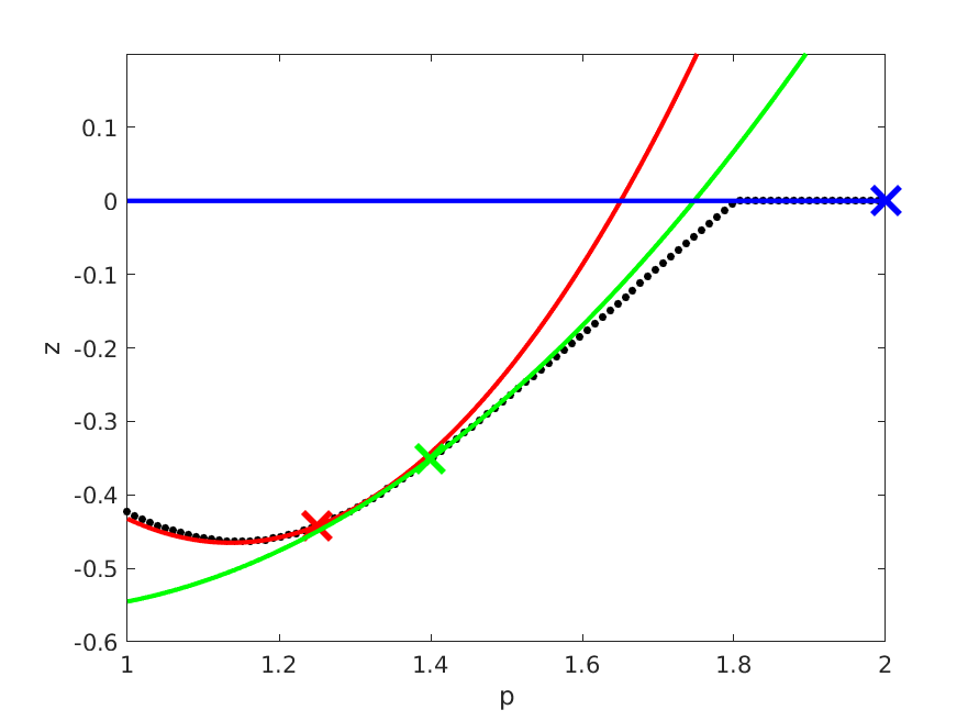
Second-order approximations to parametric solution curve for different p
Conclusion
We showed how to obtain first and second order sensitivities of the solution of a parametric NLP with respect to the parameter. The example used a single scalar parameter, but can easily be extended to multiple parameters. The rules of algorithmic differentiation apply: CasADi will just use one adjoint sweep to compute the full gradient for multiple parameters.
See our paper for mathematical details on sensitivity analysis.
Download code: code_1d.m, plot_nlp.m