Neural Networks in constrained optimization via ONNX
Estimated reading time: 7 minutesRationale
Incorporating neural networks in model predictive control has been trending for many years. A carefully crafted model of a mechanical device may benefit from a pure data-driven approach to model stick/slip friction. Human comfort may best be described by a learned model to be used as path constraints for an indoor climate system.
Solutions
Machine learning tools (unconstrained optimization) and CasADi (constrained optimization) are natural partners. They all share the language of mathematics, and in particular derivatives.
Since CasADi flexibly allows embedding any custom Functions in its computational graph, many proof-of-concepts have popped up over the years. The most mature one is probably l4casadi.
CasADi 3.8 introduces a standardized way to create a seamless coupling. We embraced ONNX, the AI industry’s exchange format for neural networks.
ONNX is meant for inference (=function evaluation) and encoding of neural networks, but it’s flexible enough to encode generic computational graphs, or indeed derivatives of neural networks.
Hello world, ONNX
Let’s consider a case of a shuttle driving around people on a bumpy road. It’s an optimal control problem with vibrations as path constraints. The vibration behaviour may be influenced by a parameter $\tau$ describing the wetness of the road:
$$ \begin{align} \displaystyle \underset{x_0,\ldots,x_N,\,u_0,\ldots,u_{N-1}} {\text{minimize}}\quad &\displaystyle \sum_{k=0}^{N-1} u_k^2 \newline \text{subject to} \, \quad & x_{k+1} = F(x_k,u_k), & k=0,\ldots,N-1 \newline & -1 \leq u_k \leq 1, & k=0,\ldots,N-1 \newline & 0 \leq v_k \leq 1.5, & k=0,\ldots,N-1 \newline & \mathrm{vibr}(x_k,\tau) \leq 0.48, & k=0,\ldots,N-1 \newline & x_0 = (0,0)^\top, \quad x_N = (1.8,0)^\top \end{align} $$
with state $x_k=(p_k,v_k)^\top$ (position, velocity), control $u_k$ the acceleration, $N=3$ and dynamics $F$.
Using CasADi Opti, this becomes:
opti = ca.Opti()
τ = opti.parameter()
opti.set_value(τ, 0)

N = 3
X = opti.variable(2, N+1)
U = opti.variable(1, N)
opti.minimize(ca.sumsqr(U))

for k in range(N):
    opti.subject_to(       X[:, k+1] == F(X[:, k], U[:, k]))
    opti.subject_to(-1 <= (U[:, k]   <= 1))
    opti.subject_to( 0 <= (X[1, k]   <= 1.5))
    opti.subject_to(vibr(X[:, k], τ) <= .48)

opti.subject_to(X[:, 0] == [0, 0])
opti.subject_to(X[:, N] == [1.8, 0])

opti.solver("ipopt")

sol = opti.solve()
Download code: step1.py
We can use torch to train a neural network and export it as onnx:
torch.onnx.export(model, (torch.zeros(1, 2, dtype=torch.float64),
                         torch.zeros(1, 1, dtype=torch.float64)), "vibr.onnx",
                  input_names=["x", "τ"], output_names=["y"],
                  dynamo=True, opset_version=18, external_data=False)
Download code: step2.py
A new CasADi construct, GraphBuilder, allows us to read that ONNX file,
possibly make some parametric dimensions concrete, and then create a CasADi Function:
vibr = ca.GraphBuilder("vibr.onnx").create("vibr")
print(vibr)
vibr:(x[1x2],τ)->(y) OnnxRuntimeInterface
This required a little extra setup: download an onnxruntime from https://github.com/microsoft/onnxruntime/releases, and make it available in the CASADI_ONNXRUNTIME_LIB environment variable:
export CASADI_ONNXRUNTIME_LIB=/path/to/onnxruntime-linux-x64-1.22.0/lib/libonnxruntime.so
It’s this library that will be in charge of evaluating the ONNX file efficiently, on a CPU or a GPU.
You can now happily evaluate this graph, just like any other CasADi Function:
print(vibr([1.0, 0.5], 0.0))
0.130223
Jacobians and Hessians
How do we get a Jacobian to work?
J = ca.jacobian(vibr(x, τ), x)
This results in an error:
Derivatives cannot be calculated for vibr
Finite differences
The lazy way is to defer to CasADi’s built-in Finite Differences:
vibr = ca.GraphBuilder("vibr.onnx").create("vibr", {"enable_fd": True})
Limited precision and speed, but may get the job done.
Now, Ipopt is happy to solve the shuttle problem in a 8.83ms. Notably, it was able to construct nlp_jac_g using a mixture of CasADi graph AD, and FD on top of the ONNX call.
      solver  :   t_proc      (avg)   t_wall      (avg)    n_eval
       nlp_f  |  16.00us (  1.23us)  13.63us (  1.05us)        13
       nlp_g  | 348.00us ( 26.77us) 341.86us ( 26.30us)        13
  nlp_grad_f  |  22.00us (  1.57us)  22.57us (  1.61us)        14
  nlp_hess_l  |  15.07ms (  1.26ms)   1.05ms ( 87.23us)        12
   nlp_jac_g  |  57.48ms (  4.11ms)   2.17ms (154.90us)        14
       total  | 132.05ms (132.05ms)   8.83ms (  8.83ms)         1
Download code: step3.py
Algorithmic differentiation
The more interesting route is to have your machine learning tool perform source-code-transforming algorithmic differentiation on the neural network and make that part of the exported ONNX file. The most efficient way is when you keep vibr.onnx for pure evaluation, and add for example adj_vibr.onnx to do reverse sensitivity sweeps.
You can now imagine CasADi-generated nlp_g talking with vibr.onnx and nlp_jac_g talking to adj_vibr.onnx.
This boils down to some sort of convention on top of the ONNX standard, tailored to constrained optimization.
If you are using torch (and in fact the whole point of the ONNX exchange standard is that you can easily model/train in some environment and load that graph in torch), there is a convenience package torch2casadi (pip install torch2casadi) that does all the required plumbing:
from torch2casadi import export

export(model, (torch.zeros(1, 2, dtype=torch.float64), torch.zeros(1, 1, dtype=torch.float64)),
       ".", name="vibr", overwrite=True, input_names=["x", "τ"], is_diff_in=[True, False])
This will generate vibr.onnx, adj_vibr.onnx, fwd_adj_vibr.onnx.
Download code: step4.py
The CasADi Function vibr will now automatically become twice differentiable. No extra options needed:
vibr = ca.GraphBuilder("vibr.onnx").create("vibr")
IPOPT solves cleanly, and a bit faster:
      solver  :   t_proc      (avg)   t_wall      (avg)    n_eval
       nlp_f  |  14.00us (  1.08us)  11.99us (921.92ns)        13
       nlp_g  |  14.36ms (  1.10ms) 357.96us ( 27.54us)        13
  nlp_grad_f  |  25.00us (  1.79us)  22.10us (  1.58us)        14
  nlp_hess_l  |  14.76ms (  1.23ms)   1.01ms ( 83.99us)        12
   nlp_jac_g  |  15.09ms (  1.08ms) 991.62us ( 70.83us)        14
       total  |  74.67ms ( 74.67ms)   4.95ms (  4.95ms)         1
Download code: step5.py
If you export the constraint Jacobian graph with ca.export_graph(ca.jacobian(opti.g, X), "step5.html") and drill down into one of the jac_wrap_vibr calls, you can see adj_vibr.onnx being embedded.
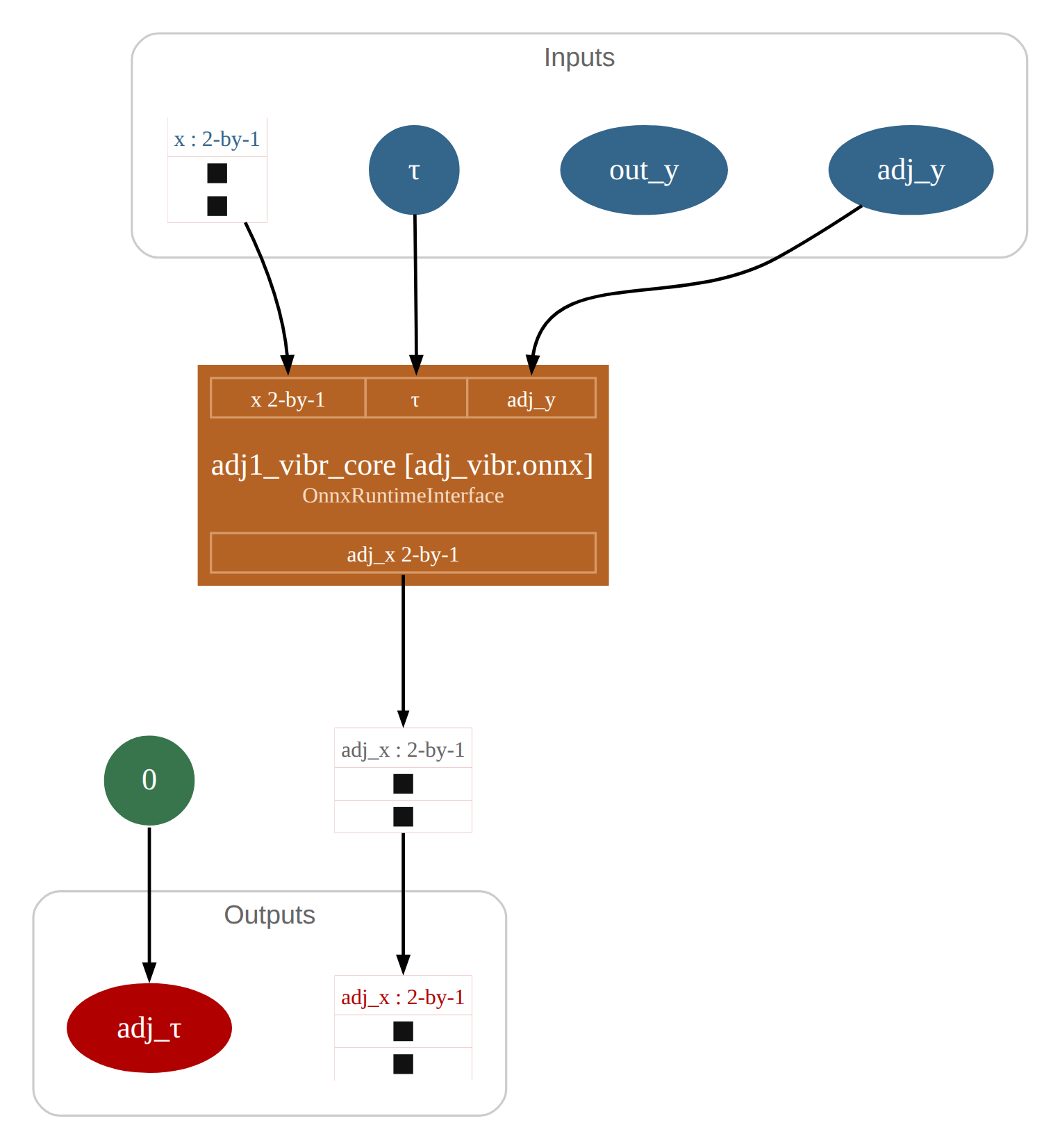
The adj_vibr.onnx call node inside CasADi's constraint Jacobian
A whitebox Neural Network
For a subset of the ONNX standard, we also allow to import models symbolically, encoding the neural network flow directly in MX.
vibr = ca.GraphBuilder("vibr.onnx").create("vibr", {"symbolic": True})
print(vibr)
vibr:(x[2],τ)->(y) MXFunction
For small Neural Networks that may be more efficient, as CasADi is optimized to work with small/medium scale heterogeneous models, as opposed to AI tools which are optimized for bulky tensor operations.
      solver  :   t_proc      (avg)   t_wall      (avg)    n_eval
       nlp_f  |  10.00us (769.23ns)   7.12us (547.92ns)        13
       nlp_g  |  66.00us (  5.08us)  64.30us (  4.95us)        13
  nlp_grad_f  |  14.00us (  1.00us)  13.73us (980.71ns)        14
  nlp_hess_l  |  94.00us (  7.83us)  94.22us (  7.85us)        12
   nlp_jac_g  | 173.00us ( 12.36us) 173.52us ( 12.39us)        14
       total  |   2.26ms (  2.26ms)   2.26ms (  2.26ms)         1
Download code: step7.py
Adapting weights
Another use-case is to fine-tune or fit the NN weights inside a CasADi optimization. There is no technical restriction in the ONNX standard or the CasADi interface to develop such a case. In torch, you can promote weights into updatable parameters with:
class FreeWeights(nn.Module):
    def __init__(self, model):
        super().__init__()
        self.model = model
        self.names = [n for n, _ in model.named_parameters()]

    def forward(self, *args):
        n = len(self.names)
        return torch.func.functional_call(self.model, dict(zip(self.names, args[-n:])), args[:-n])

params = [p.detach() for p in model.parameters()]
export(FreeWeights(model), (torch.zeros(1, 2, dtype=torch.float64),
                            torch.zeros(1, 1, dtype=torch.float64), *params), ".",
       name="vibr", input_names=["x", "τ", "W1", "b1", "W2", "b2"], hessian=False, overwrite=True)
vibr = ca.GraphBuilder("vibr.onnx").create("vibr")
print(vibr)
vibr:(x[2],τ,W1[48],b1[16],W2[16],b2)->(y) OnnxRuntimeInterface
The solvers shipped in CasADi are not specifically tailored to NN (they are tailored to constrained optimization), so two caveats apply: avoid using non-smooth activation functions, and avoid using exact Hessians
(hessian=False skips exporting the forward-over-adjoint graph, whose cost grows with the number of weights).
Other than that, you can just proceed like:
opti = ca.Opti()
weights = [opti.variable(p.numel()) for p in params]
residuals = ca.vertcat(*[vibr(m[:2], m[2], *weights) - y for m, y in zip(meas, y_meas)])
opti.minimize(ca.sumsqr(residuals)
              + 1e-2*sum(ca.sumsqr(w-p.reshape(-1).numpy()) for w, p in zip(weights, params)))
for w, p in zip(weights, params):
    opti.set_initial(w, p.reshape(-1).numpy())
opti.solver("ipopt", {}, {"hessian_approximation": "limited-memory",
                          "limited_memory_max_history": 50})
sol = opti.solve()
Here, meas and y_meas are 64 vibration measurements taken on the actual shuttle, which turns out to vibrate a bit more than the pretraining data suggested.
The fit starts from the pretrained weights and stays close to them:
RMS error before: 0.1536804668330229
RMS error after:  0.010159448309198394
Download code: step8.py
Future work
It may be interesting to perform source-code-transforming AD on ONNX standalone without a dependency on pytorch. An experimental package can be found at onnx-ad
Wrap-up
This new feature of CasADi is still in its infancy, but I believe our progressive embracing of the ONNX standard will open a lot of possibilities in the future whilst avoiding vendor lock-in for your team of engineers. As a bonus, all of the above is compatible with CasADi C code generation.
Enjoy!
A video recording of this blog post’s content is available: