Parfor

In this post we’ll explore how to use Matlab’s parfor with a CasADi nonlinear program.

The nonlinear program (NLP) of interest is the following: $$ \begin{align} \displaystyle \underset{x,y} {\text{minimize}}\quad &\displaystyle (1-x)^2+(y-x^2)^2 \newline \text{subject to} \, \quad & x^2+y^2 \leq r \end{align} $$ Note that $r$ is a free parameter. Our goal is to collect each solution of the NLP as we loop over $r$. We could imagine performing such task when tracing a pareto front of a multi-objective optimization, for which the parameter would be the a weight to combine those objectives.

Problem construction inside the loop

The first way to work with parfor and CasADi is to do the problem construction entirely in the loop:

N = 250;

fsol = zeros(1,N);
rs = linspace(1,3,N);

parfor i=1:N
  r = rs(i);
  x = casadi.SX.sym('x');
  y = casadi.SX.sym('y');

  v = [x;y];
  f = (1-x)^2+(y-x^2)^2;
  g = x^2+y^2;
  nlp = struct('x', v, 'f', f, 'g', g);

  % Create IPOPT solver object
  solver = casadi.nlpsol('solver', 'ipopt', nlp);

  % Solve the NLP
  res = solver('x0' , [2.5 3.0],...      % solution guess
               'lbx', -inf,...           % lower bound on x
               'ubx',  inf,...           % upper bound on x
               'lbg', -inf,...           % lower bound on g
               'ubg',  r);               % upper bound on g
   
  
  % Store the solution
  fsol(i) = full(res.f);
end

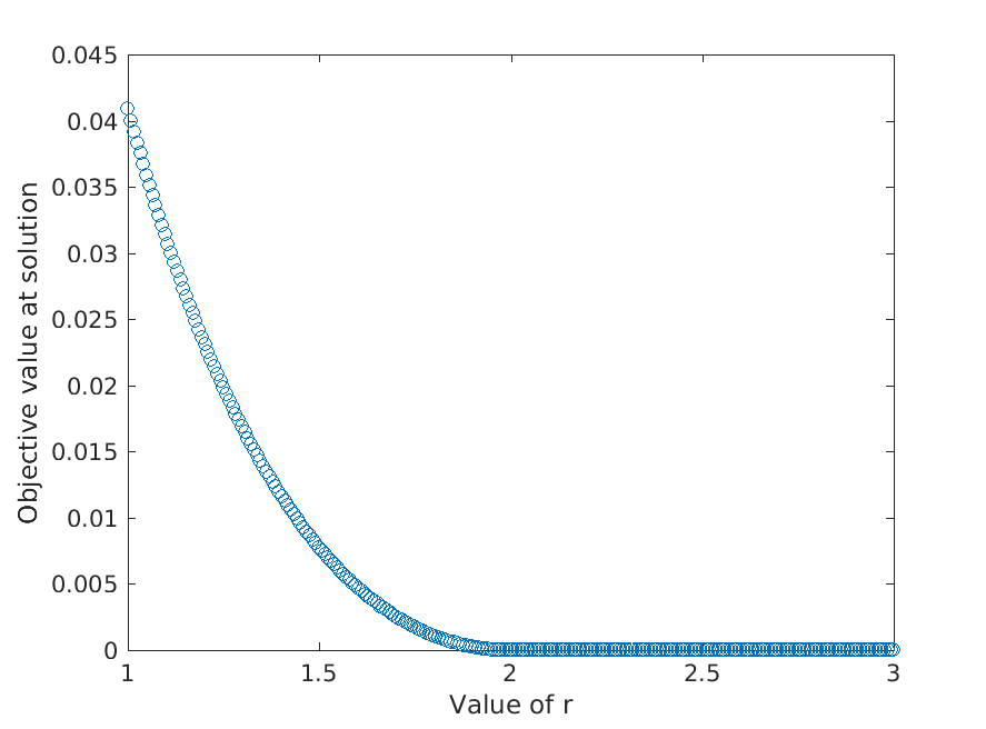
plot(rs,fsol,'o')

We obtain a nice plot:

Download code: casadi_parfor1.m

Problem construction outside the loop

Constructing CasADi expressions and Functions incurs an initialization cost. Therefore, we always advise to construct the solver fully outside of the loop, and simply make numerical calls to it in the loop.

This advice collided with our limited support for parfor so far. CasADi 3.5 comes with improved support. The loop body may now contain numerical calls to CasADi Functions defined outside that loop:

x = casadi.SX.sym('x');
y = casadi.SX.sym('y');

v = [x;y];
f = (1-x)^2+(y-x^2)^2;
g = x^2+y^2;
nlp = struct('x', v, 'f', f, 'g', g);

% Create IPOPT solver object
solver = casadi.nlpsol('solver', 'ipopt', nlp);

tic
parfor i=1:N
  % Solve the NLP
  res = solver('x0' , [2.5 3.0],...      % solution guess
               'lbx', -inf,...           % lower bound on x
               'ubx',  inf,...           % upper bound on x
               'lbg', -inf,...           % lower bound on g
               'ubg',  rs(i));           % upper bound on g
   
  
  % Store the solution
  fsol(i) = full(res.f);
end
toc

plot(rs,fsol,'o')

Download code: casadi_parfor2.m

Note 1: for this example the parameter entered trivially through ‘ubg’. In general, you may need to work with a parametric NLP:

p = casadi.SX.sym('p');
g = x^2+y^2-p;
nlp = struct('x', v, 'p', p, 'f', f, 'g', g);

  res = solver('x0' , [2.5 3.0],...      % solution guess
               ...
               'p',  rs(i));

Note 2: constructing CasADi Functions inside the loop with CasADi symbols declared outside the loop is forbidden, but inefficient anyway.

Implementation details and Python

We did not actually code anything parfor-specific in CasADi. The reason that CasADi 3.5 supports the construct above now is because we implemented serialization/deserialization of CasADi Functions.

Parfor uses this under the hood to transfer problems/results to/from different threads. Such mechanism is often encounter for parallelization, for example in Python’s multiprocessing module. In fact, the above code can easily be rewritten for Python:

from multiprocessing import Pool

from casadi import *

N = 250
rs = np.linspace(1,3,N)

x = SX.sym('x')
y = SX.sym('y')

v = vertcat(x,y)
f = (1-x)**2+(y-x**2)**2
g = x**2+y**2
nlp = {'x': v, 'f': f, 'g': g}

# Create IPOPT solver object
solver = casadi.nlpsol('solver', 'ipopt', nlp)

def optimize(r):
  res = solver(x0=[2.5,3.0],      # solution guess
               lbx=-inf,          # lower bound on x
               ubx=inf,           # upper bound on x
               lbg=-inf,          # lower bound on g
               ubg=r)         # upper bound on g
   
  
  return float(res["f"])

b = Pool(2)
fsol = b.map(optimize, rs)

Download code: casadi_multiprocessing.py

In conclusion, we demonstrated a new way to solve NLPs in parallel with CasADi. Finally, note that we have an unrelated parallelization mechanism to evaluate e.g. constraints of a single NLP in parallel.