Tensorflow and CasADi
Estimated reading time: 5 minutesIn this post we’ll explore how to couple Tensorflow and CasADi. Thanks to Jonas Koch (student @ Applied Mathematics WWU Muenster) for delivering inspiration and example code.
One-dimensional regression with GPflow
An important part of machine learning is about regression: fitting a (non-)linear model through sparse data. This is an unconstrained optimization problem for which dedicated algorithms and software are readily available.
Let’s create some datapoints to fit, a perturbed sine.
data = np.linspace(0,10,N).reshape((N,1))
value = np.sin(data)+np.random.normal(0,0.1,(N,1))
We make use of GPflow, software which is built on top of Tensorflow, to perform a Gaussian process regression:
model = gpflow.models.GPR(data, value, gpflow.kernels.Constant(1) + gpflow.kernels.Linear(1) + gpflow.kernels.White(1) + gpflow.kernels.RBF(1))
gpflow.train.ScipyOptimizer().minimize(model)
The trained model has a predict_y method to deliver us the mean and variance of the fit at any location(s):
xf = np.linspace(0,10,10*N).reshape((-1,1))
[mean,variance] = model.predict_y(xf)
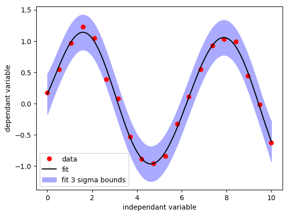
1D regression example with GPflow
Embedding the regression model in a CasADi graph
The mechanism for embedding foreign code in CasADi is through the use of a Callback:
class GPR(Callback):
  def __init__(self, name,  opts={}):
    Callback.__init__(self)
    self.construct(name, opts)

  def eval(self, arg):
    [mean,_] = model.predict_y(np.array(arg[0]))
    return [mean]
After instantiating the Callback, we end up with a plain-old CasADi function object which we can evaluate numerically or symbolically. One caveat, the user is responsible of keeping at least one reference to this Function.
gpr = GPR('GPR', {"enable_fd":True})
As an example of embedding, we can ask Ipopt to compute the minimum of this function. Finite differences will be used to differentiate the Callback:
x = MX.sym("x")
solver = nlpsol("solver","ipopt",{"x":x,"f":gpr(x)})
res = solver(x0=5)
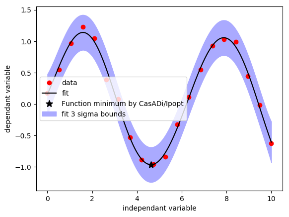
1D regression example with GPflow
Download code: gpflow_example.py
Optimal control example (slow)
The GPR model from the previous paragraph was a mapping from $R$ to $R$. To make things more interesting, we will increase the dimension to a mapping from $R^\textrm{nd}$ to $R$.
I didn’t have much inspiration to come up with high-dimensional data to fit, so these random arrays will have to do. Of course, it’s rather silly to fit a model through purely random data..
data = np.random.normal(loc=0.5,scale=1,size=(N,nd))
value = np.random.random((N,1))
model = gpflow.models.GPR(data, value, gpflow.kernels.Constant(nd) + gpflow.kernels.Linear(nd) + gpflow.kernels.White(nd) + gpflow.kernels.RBF(nd))
Our callback will need to override the default-scalar sparsity for its input:
class GPR(Callback):
  def __init__(self, name,  opts={}):
    ...

  def get_sparsity_in(self,i):
      return Sparsity.dense(nd,1)
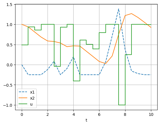
For the remainder, we will just use the code of CasADi’s direct_multiple_shooting example, but the solver construction is modified as follows.
The objective is replace by our nd-dimensional model evaluated on the concatenation of all x-states over the optimal control horizon.
We use a limited-memory Hessian approximation here to avoid the cost of obtaining second-order sensitivities.
w = vertcat(*w)

prob = {'f': gpr(w[0::3]), 'x': w , 'g': vertcat(*g)}
options = {"ipopt": {"hessian_approximation": "limited-memory"}}
solver = nlpsol('solver', 'ipopt', prob,options);
The problem takes quite some time to solve.
If you look at the timings printout, you’ll see that in particular the cost of computing the gradient of the objective (nlp_grad_f) is excessive:
               t_proc [s]   t_wall [s]    n_eval
       nlp_f        0.291        0.261        31
       nlp_g       0.0079      0.00789        31
  nlp_grad_f         25.7         23.2        32
   nlp_jac_g       0.0496       0.0502        32
      solver         26.2         23.6         1
If you insert a print statement to inspect the arguments at our Callback’s eval method, you’ll see the finite differences happening live in your terminal:
each of the nd inputs to gpr is individually perturbed, making the cost to compute the gradient of the objective nd times more expensive than the cost of just the objective.
The solution requires 2783 calls to our Callback, and the Callback ran for a total of 21.7 seconds.
Optimal control example (slow)
Download code: ocp.py
Optimal control example (fast)
We’ll speed up our code on two fronts:
First, we notice that predict_y incurs quite some overhead. Instead of calling it repeatedly, let’s work with the underlying Tensorflow graphs:
X = tf.placeholder(shape=(1,nd),dtype=np.float64)
[mean,_] = model._build_predict(X)
Running this mean graph in a tensorflow session has much less overhead:
import tensorflow as tf
with tf.Session() as session:
  session.run(mean, feed_dict(X: np.array(...)))
Second, we notice that tensorflow supports algorithmic differentation. If we add a reverse mode implementation to our Callback, we can get the gradient for (a small multiple of) the cost of the objective. Note that (vanilla) Tensorflow offers only the reverse mode of AD, not the forward mode. This is logical, since it focusses on unconstrained optimization.
It’s quite easy to create a general purpose TensorFlowEvaluator Callback (tensorflow_casadi.py for full code):
class TensorFlowEvaluator(casadi.Callback):
  def __init__(self,t_in,t_out,session, opts={}):
    ....

  def eval(self,arg):
    # Associate each tensorflow input with the numerical argument passed by CasADi
    d = dict((v,arg[i].toarray()) for i,v in enumerate(self.t_in))
    # Evaluate the tensorflow expressions
    ret = self.session.run(self.t_out,feed_dict=d)
    return ret

  def has_reverse(self,nadj): return nadj==1
  def get_reverse(self,nadj,name,inames,onames,opts):
    # Construct tensorflow placeholders for the reverse seeds
    adj_seed = [tf.placeholder(shape=self.sparsity_out(i).shape,dtype=tf.float64) for i in range(self.n_out())]
    # Construct the reverse tensorflow graph through 'gradients'
    grad = tf.gradients(self.t_out, self.t_in,grad_ys=adj_seed)
    # Create another TensorFlowEvaluator object
    callback = TensorFlowEvaluator(self.t_in+adj_seed,grad,self.session)
    ...
With these two modifications in place, the solution requires just 63 calls to our Callback, for a total Callback runtime of 0.13 seconds.
Download code: ocp_faster.py, tensorflow_casadi.py
In conclusion, we’ve shown how to embed calls to foreign code in CasADi graphs. Though the optimal control example is contrived, it conveys how such coupling can be made efficient.
To learn more ways to endow sensitivity-information on a Callback, see the callback.py example.