Optimal control problems in a nutshell
Estimated reading time: 5 minutesOptimization. There’s a mathematical term that sounds familiar to the general public. Everyone can imagine engineers working hard to make your car run 1% more fuel-efficient, or to slightly increase profit margins for a chemical company.
That sounds rather dull; an icing on the cake at best. Optimization can be more than this. I’d argue that optimization can deliver intelligence or creativity.
Consider that finding your next chess move amounts to optimization. Consider the results of topology optimization
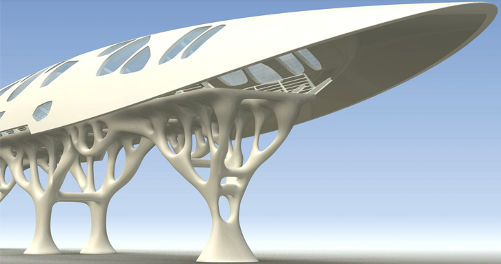
Topology optimization
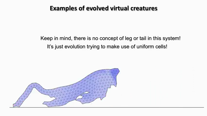
Evolving artificial life
Our field of research is optimal control, in which we seek time-trajectories for control signals that make a dynamic system carry out a task in an optimal way.
In many cases, like for a double pendulum swing-up
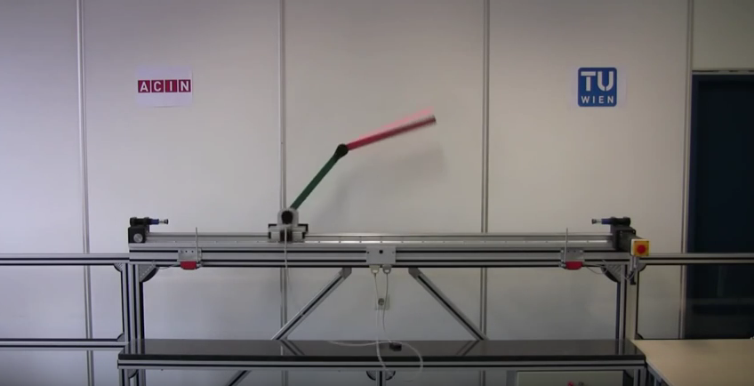
Double pendulum
the most exciting part of optimal control is not that it can spot the optimum out of many valid trajectories. It’s that it can find valid trajectories at all, out of the blue.
Slot car racing problem
Let’s get concrete and solve an actual optimal control problem, using CasADi. We will go racing a toy slot car.
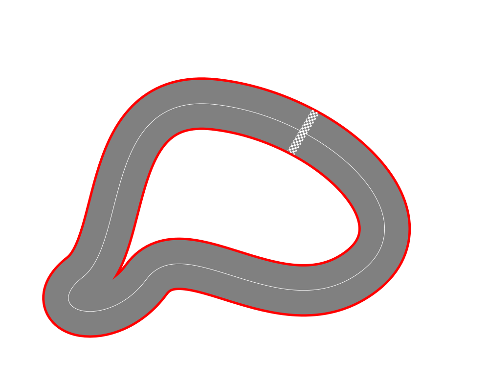
Race track
The task is to finish 1 lap as fast as possible, starting from standstill. Go too fast, and the car will fly out of its slot. There is just one way to control the system: pick the amount of throttle $u(t)$ at any give time.
First, we encode the knowledge we have about the system dynamics in a differential equation (ODE):
$$ \frac{d \begin{bmatrix} p(t) \ v(t) \end{bmatrix}}{dt} = \begin{bmatrix} v(t) \ u(t)-v(t) \end{bmatrix}, $$ where $p(t)$ is position and $v(t)$ is speed.
Summarizing the system states in one vector $x(t) = [p(t);v(t)]$, we have: $$ \dot{x}(t) = f(x(t),u(t)). $$
Next, we encode the the task definition in a continuous-time optimal control problem (OCP).
$$ \begin{align} \displaystyle \underset{\begin{array}{c}x(\cdot), u(\cdot)\end{array}} {\text{minimize}}\quad &\displaystyle T \newline \text{subject to} \, \quad & \dot{x}(t) = f(x(t),u(t)) \quad t \in [0,T], & \textrm{dynamic constraints} \newline & p(0) = 0, & \textrm{boundary condition: start at position 0} \newline & v(0) = 0, & \textrm{boundary condition: start with zero speed}\newline & p(T) = 1, & \textrm{boundary condition: the finish line is at position 1}\newline & 0 \leq u(t) \leq 1, & \textrm{path constraint: throttle is limited} \newline & v(t) \leq L(p(t)). & \textrm{path constraint: speed limit varying along the track} \newline \end{align} $$
Note our decision variables $x(\cdot)$ and $u(\cdot)$: the result of the optimization should be functions, i.e. infinitely detailed descriptions of how the states and control should move over time from $0$ to $T$:
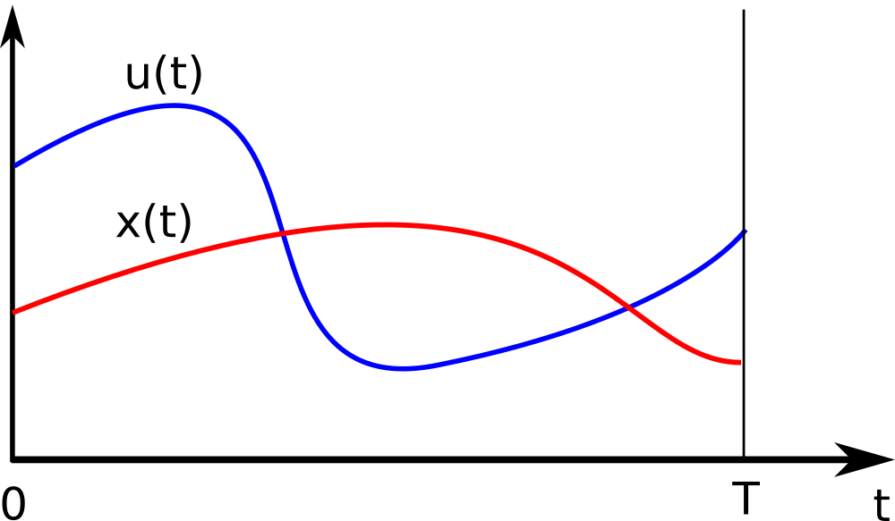
Continuous-time states and controls
Multiple-shooting
Computers don’t like infinities. Therefore, let’s discretize the problem in time. Choose a number $N$ of control intervals in which the control effort is kept constant:
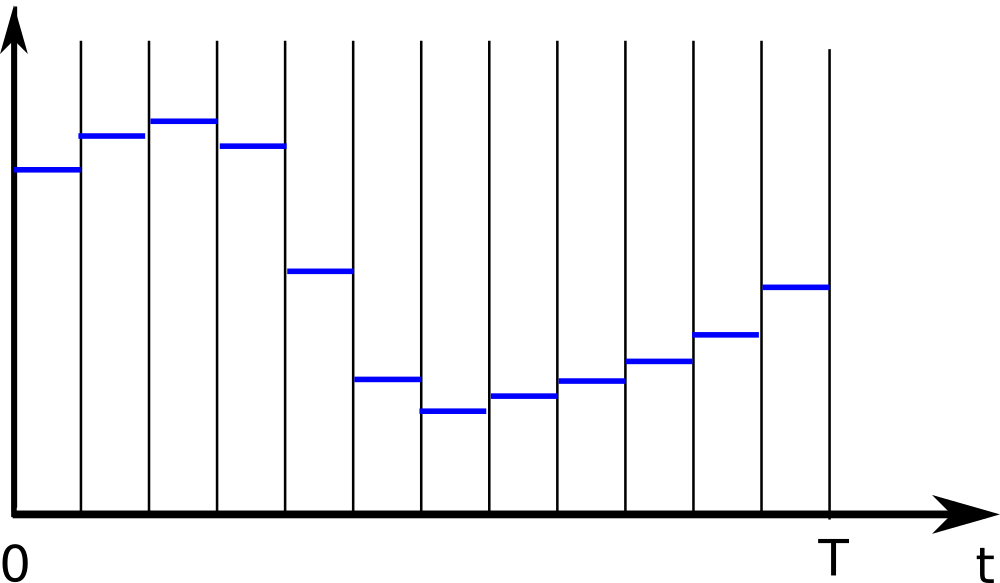
Discretized controls
We now have decision variables $u_1,u_2,\ldots,u_{N}$ instead of function $u(\cdot)$.
For the state trajectory, let’s consider the states at the boundaries of each control interval:
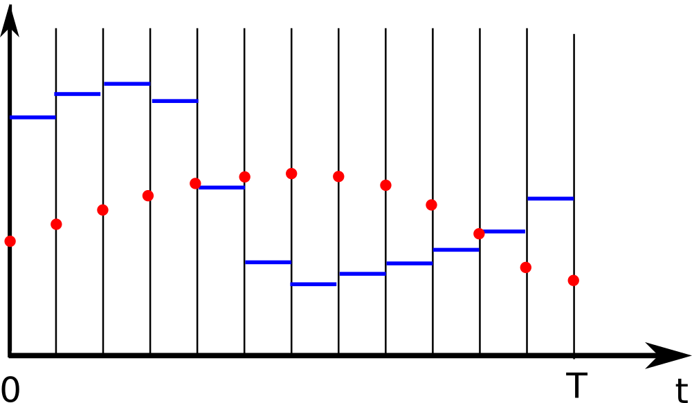
Discretized states and controls
We now have decision variables $x_1,x_2,\ldots,x_{N+1}$ instead of function $x(\cdot)$.
In each control interval $k$, we now have a start state $x_k$ and a fixed control signal $u_k$. Over this interval, we may perform a time integration of our ODE. For example, using explicit euler: $x_{k+1} \approx x_{k} + \frac{T}{N} f(x_k,u_k)$, in general:
$$ x_{k+1} = F(x_k,u_k). $$
For each interval the integrator predicts were our system will end up at the end of that interval. Starting our numerical optimization with putting all states at a constant location, the picture may look like:
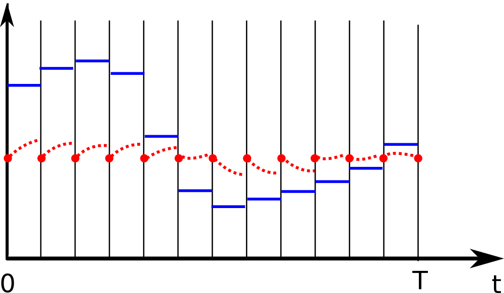
Gaps
We notice gaps here; there’s a mismatch between were the integrator says we will end up and where our state decision variables think we are. What we do is add constraints that make the gap zero.
The result is a multiple-shooting transcription of the original OCP:
$$ \begin{align} \displaystyle \underset{u_1,u_2,\ldots,u_{N},x_1,x_2,\ldots,x_{N+1}} {\text{minimize}}\quad &\displaystyle T \newline \text{subject to} \, \quad & x_{k+1} = F(x_k,u_k) \quad k=1 \ldots N, & \textrm{dynamic constraints a.k.a. gap closing} \newline & p_1 = 0, & \textrm{boundary condition: start at position 0} \newline & v_1 = 0, & \textrm{boundary condition: start with zero speed}\newline & p_{N+1} = 1, & \textrm{boundary condition: the finish line is at position 1}\newline & 0 \leq u_k \leq 1, \quad k=1 \ldots N , & \textrm{path constraint: throttle is limited} \newline & v_k \leq L(p_k). \quad k=1 \ldots N+1 & \textrm{path constraint: speed limit varying along the track} \newline \end{align} $$
Coding
Let’s get coding, using CasADi’s Opti functionality.
Set up the problem
N = 100; % number of control intervals

opti = casadi.Opti(); % Optimization problem
Declare decision variables.
X = opti.variable(2,N+1); % state trajectory
pos   = X(1,:);
speed = X(2,:);
U = opti.variable(1,N);   % control trajectory (throttle)
T = opti.variable();      % final time
Set the objective.
opti.minimize(T); % race in minimal time
Specify system dynamics.
f = @(x,u) [x(2);u-x(2)]; % dx/dt = f(x,u)
Create gap closing constraints, picking Runge-Kutta as integration method.
dt = T/N; % length of a control interval
for k=1:N % loop over control intervals
   % Runge-Kutta 4 integration
   k1 = f(X(:,k),         U(:,k));
   k2 = f(X(:,k)+dt/2*k1, U(:,k));
   k3 = f(X(:,k)+dt/2*k2, U(:,k));
   k4 = f(X(:,k)+dt*k3,   U(:,k));
   x_next = X(:,k) + dt/6*(k1+2*k2+2*k3+k4);
   opti.subject_to(X(:,k+1)==x_next); % close the gaps
end
Set path constraints.
limit = @(pos) 1-sin(2*pi*pos)/2;
opti.subject_to(speed<=limit(pos)); % track speed limit
opti.subject_to(0<=U<=1);           % control is limited
Set boundary conditions.
opti.subject_to(pos(1)==0);   % start at position 0 ...
opti.subject_to(speed(1)==0); % ... from stand-still
opti.subject_to(pos(N+1)==1); % finish line at position 1
One extra constraint.
opti.subject_to(T>=0); % Time must be positive
Provide initial guesses for the solver:
opti.set_initial(speed, 1);
opti.set_initial(T, 1);
Solve the NLP using IPOPT
opti.solver('ipopt'); % set numerical backend
sol = opti.solve();   % actual solve
Post processing of the optimal values.
plot(sol.value(speed));
plot(sol.value(pos));
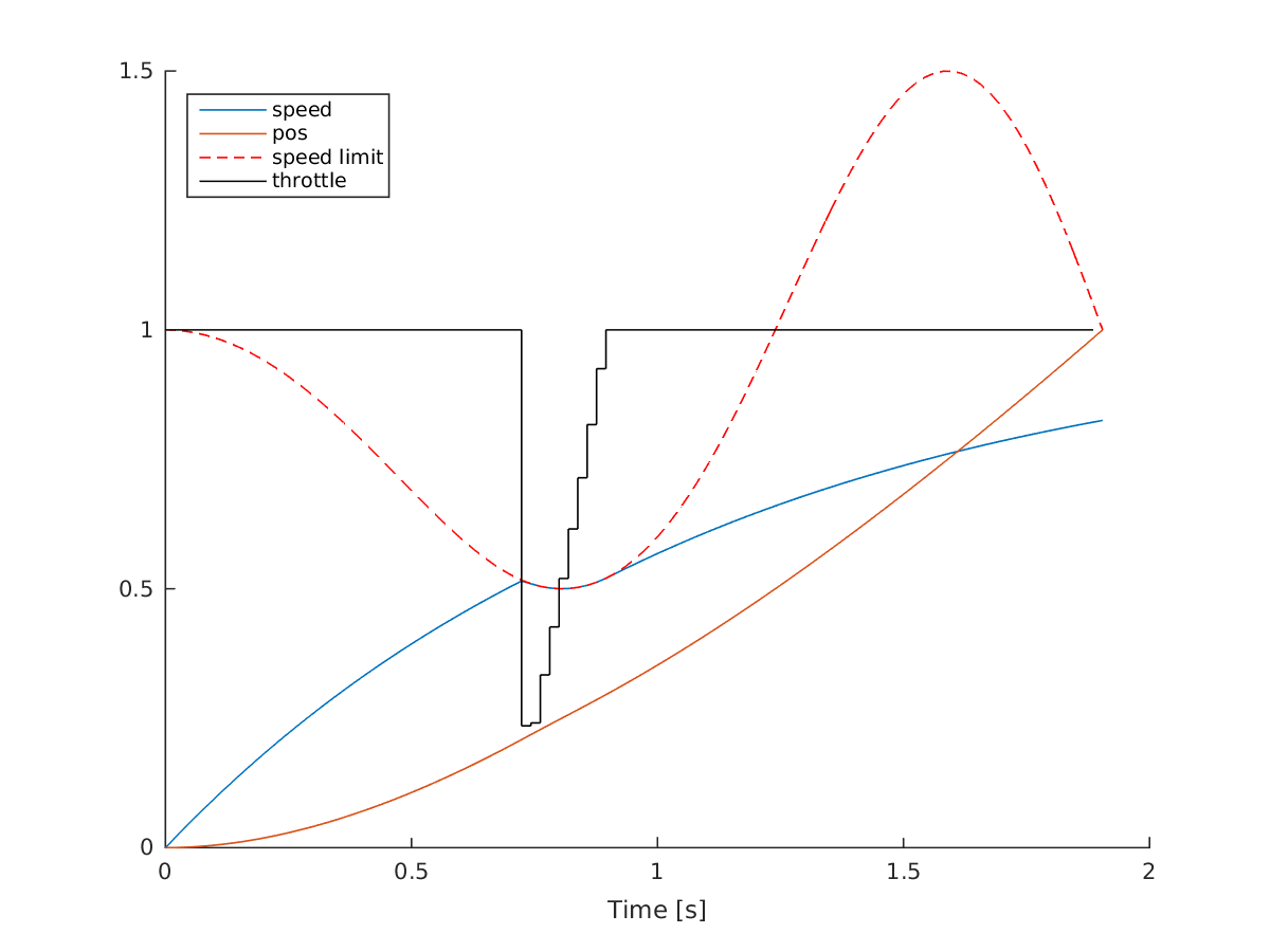
Solution of race car problem
The solution is intuitive: we give 100% throttle, until we hit the speed limit. Next, we gradually inrease throttle again as the speed limit is raised.
A characteristic of the multiple-shooting approach is that there are many optimization variables (much more than in single-shooting), but there is a lot of sparsity in the problem.
Indeed, have a look at the sparsity of the constraint Jacobian:
spy(sol.value(jacobian(opti.g,opti.x)))
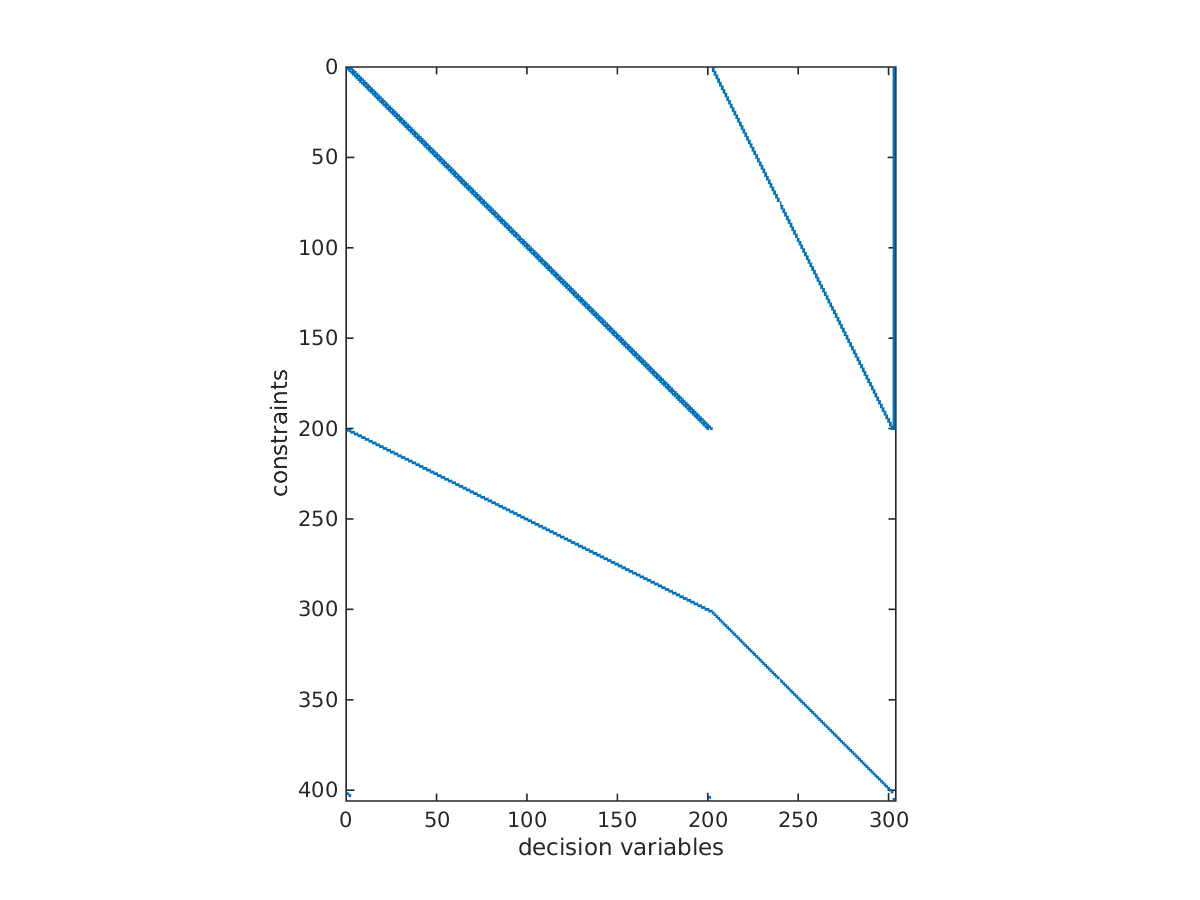
Sparsity of constraint jacobian
This structure is automatically detected and exploited by CasADi.
Download code: race_car.m