Easy NLP modeling in CasADi with Opti
Estimated reading time: 3 minutesRelease 3.3.0 of CasADi introduced a compact syntax for NLP modeling, using a set of helper classes, collectively known as ‘Opti stack’.
In this post, we briefly demonstrates this functionality.
Rosenbrock problem
Let’s consider the classic Rosenbrock problem to begin with:
$$ \begin{align} \displaystyle \underset{x,y} {\text{minimize}}\quad &\displaystyle (1-x)^2+(y-x^2)^2 \ \end{align} $$
In CasADi’s Opti syntax, we can easily transcribe this to computer code:
opti = casadi.Opti();

x = opti.variable();
y = opti.variable();

opti.minimize((1-x)^2+(y-x^2)^2);

opti.solver('ipopt');
sol = opti.solve();

plot(sol.value(x),sol.value(y),'o');
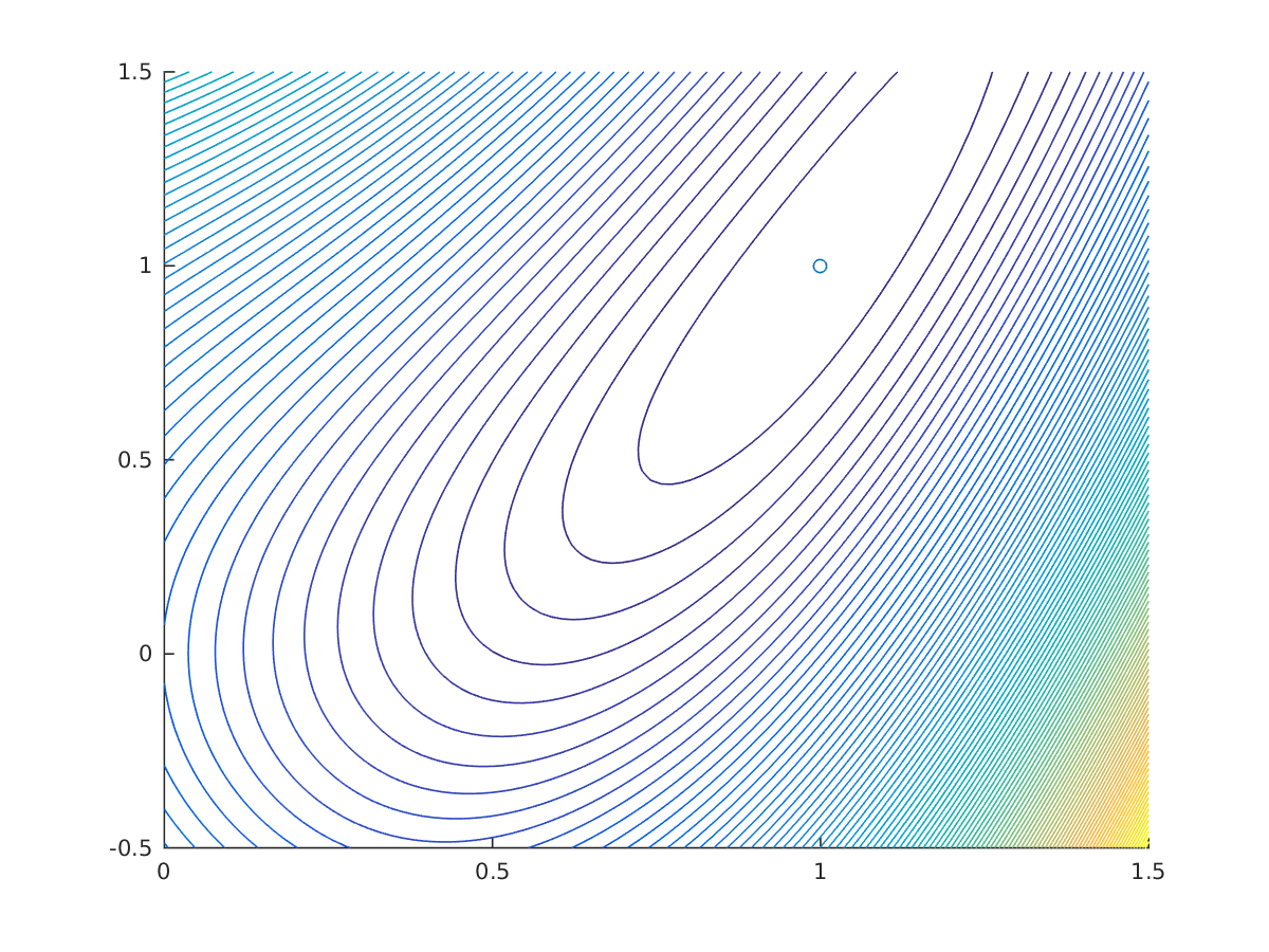
Solution of unconstrained Rosenbrock problem
Let’s make a variation on the problem by adding an equality constraint:
$$ \begin{align} \displaystyle \underset{x,y} {\text{minimize}}\quad &\displaystyle (1-x)^2+(y-x^2)^2 \newline \text{subject to} \, \quad & x^2+y^2=1 \end{align} $$
opti.minimize((1-x)^2+(y-x^2)^2);
opti.subject_to(x^2+y^2==1);

opti.solver('ipopt');
sol = opti.solve();
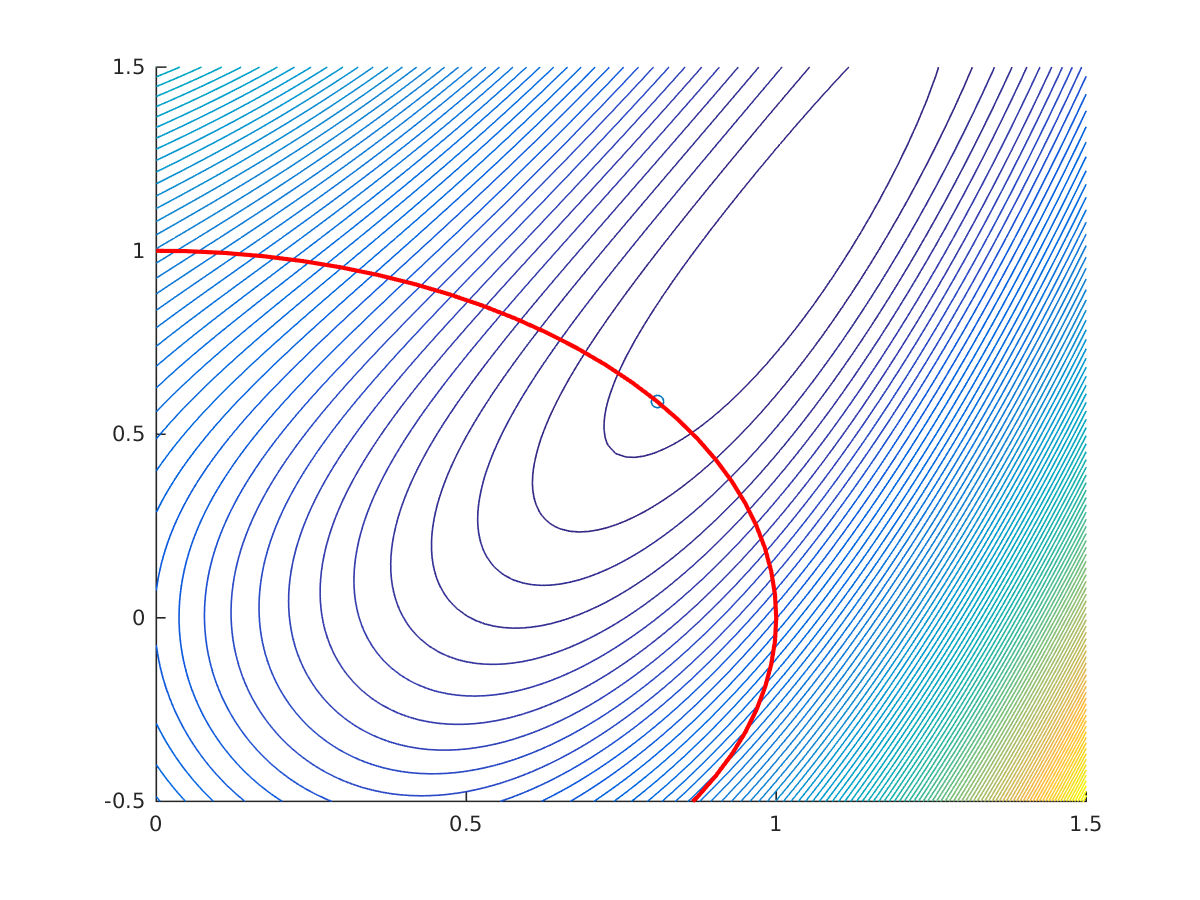
Solution of constrained Rosenbrock problem
We may add in fact any number of equality/inequality constraints:
$$ \begin{align} \displaystyle \underset{x,y} {\text{minimize}}\quad &\displaystyle (1-x)^2+(y-x^2)^2 \newline \text{subject to} \, \quad & x^2+y^2=1 \newline & y\geq x \end{align} $$
opti.minimize((1-x)^2+(y-x^2)^2);
opti.subject_to(x^2+y^2==1);
opti.subject_to(y>=x);

opti.solver('ipopt');
sol = opti.solve();
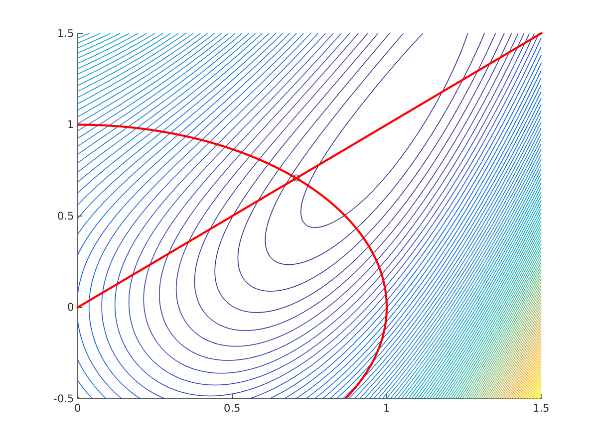
Solution of constrained Rosenbrock problem
We can also create a parametric NLP, were a parameter is getting fixed at solution time:
opti = casadi.Opti();

x = opti.variable();
y = opti.variable();
r = opti.parameter();

opti.minimize((1-x)^2+(y-x^2)^2);
con = x^2+y^2<=r;
opti.subject_to(con);
opti.solver('ipopt');

for r_value=linspace(1,3,25)
    opti.set_value(r,r_value)
    sol = opti.solve();
    plot(r_value,sol.value(f),'ko')
end
We may access the value of the Lagrange multiplier associated with the constraint using:
sol.value(opti.dual(con))
The Lagrange multiplier can be interpreted as the sensitivity of the optimal cost with respect to the relaxation of the constraint. We plotted the slope given by the Langrange multiplier in red in the figure below.
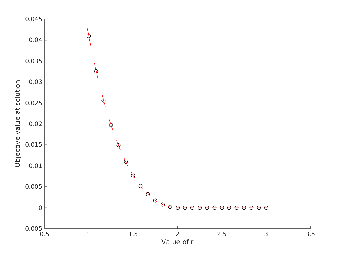
Solution of constrained Rosenbrock problem
Download code: rosenbrock.m
Hanging chain problem
Next, we will visit the hanging chain problem. We consider $N$ point masses, connected by springs, hung from two fixed points at $(-2,1)$ and $(2,1)$, subject to gravity.
We seek the rest position of the system, obtained by minimizing the total energy in the system.
Consider that point mass $i$ has position $(x_i,y_i)$, we can write the gravitational potential energy as
$$ V_g = g m \sum_{i=1}^N y_i, $$
and the total spring potential energy as:
$$ V_s = \frac{1}{2} \sum_{i=1}^{N-1} D \left((x_i-x_{i+1})^2+(y_i-y_{i+1})^2\right). $$
We can do this in Opti using a oneliner, or a for loop:
opti = casadi.Opti();

p = opti.variable(2,N);
x = p(1,:);
y = p(2,:);

V = 0.5*D*sum((x(1:N-1)-x(2:N)).^2+(y(1:N-1)-y(2:N)).^2);
V = V + g*sum(m*y);

opti.minimize(V);

opti.subject_to(p(:,1)==[-2;1])
opti.subject_to(p(:,end)==[2;1])

opti.solver('ipopt');
sol = opti.solve();

plot(sol.value(x),sol.value(y),'-o')
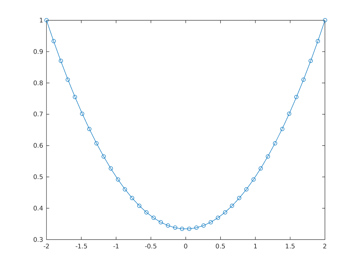
Solution of unconstrained hanging chain problem
After a first solve, further constraints can be added, e.g. a ground constrained
opti.subject_to(y>=cos(0.1*x)-0.5);
sol = opti.solve();
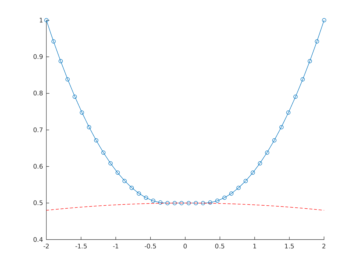
Solution of constrained hanging chain problem
We can make the problem more numerically challenging by setting a nonzero restlength for the spring:
V = 0.5*sum(D*(sqrt((x(1:N-1)-x(2:N)).^2+(y(1:N-1)-y(2:N)).^2)-L/N).^2);
V = V + g*sum(m*y);

opti.minimize(V);
When the problem is nonconvex it’s always a good idea to provide initial guesses for your decision variables:
opti.set_initial(x,linspace(-2,2,N));
opti.set_initial(y,1);
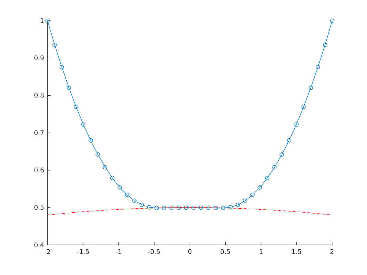
Solution of nonlinear constrained hanging chain problem
When the going get’s tough, you may find it helpful to plot the intermediate solution for each iteration of the solver:
opti.callback(@(i) plot(opti.debug.value(x),opti.debug.value(y),'DisplayName',num2str(i)))
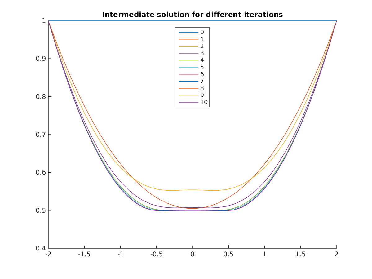
Solution of nonlinear constrained hanging chain problem
(Credits to Milan Vukov for delivering this problem)
Download code: chain.m
For more details about Opti, see Chapter 9 of the users guide. For an optimal control example, see the race car example.
Using Opti, you have the scalability of CasADi algorithmic differentiation available, in a user friendly packaging. Ideal for teaching!